Notice
This post is a free form translation (with some clarifications) of my post in Russian published on techrocks.ru. So if you know Russian, you are welcome to read it there. Otherwise, I invite you to join me here and have some fun.
Introduction
All of us solve a “shortest path” problem many times a day. Unintentionally of course. We solve it on our way work or when we browse the Internet or when we arrange our things on a desk.
Sounds a bit… too much? Let’s find out.
Imagine, you have decided to meet with friends, well … let’s say in cafe. First of all, you need to find a route (or path) to cafe, so you start looking for available public transport (if you are on foot) or routes and streets (if you are driving). You are looking for a route from your current location to cafe but not “any” route – the shortest or fastest one.
Here is a one more example, which isn’t so obvious as the previous one. During you way work you decide to take a “short cut” through a side street because well… it is a “short cut” and it is “faster” to go this way. But how did you know this “short cut” is faster? Based on personal experience you solved a “shortest path” problem and selected a route, which goes through the side street.
In both examples, the “shortest” route is determined in either distance or time required to get from one place to another. Traveling examples are very natural applications of graph theory and “shortest path” problem in particular. However, what about the example with arranging things on a desk? In this case the “shortest” can represent a number or complexity of actions you have to perform to get, for example, a sheet of paper: open desk, open folder, take a sheet of paper vs take a sheet of paper right from desk.
All of the above examples represent a problem of finding a shortest path between two vertexes in a graph (a route or path between two places, a number of actions or complexity of getting a sheet of paper from one place or another). This class of shortest path problems is called SSSP (Single Source Shortest Path) and the base algorithm for solving these problems is Dijkstra’s algorithm, which has a O(n2) computational complexity.
But, sometimes we need to find all shortest paths between all vertexes. Consider the following example: you are creating a map for you regular movements between home, work and theatre. In this scenario you will end up with 6 routes: work -> home, home -> work, work -> theatre, theatre -> work, home -> theatre and theatre -> home (the reverse routes can be different because of one-way roads for example).
Adding more place to the map will result in a significant grow of combinations – according to permutations of n formula of combinatorics it can be calculated as:
A(k, n) = n! / (n - m)!

// where n - is a number of elements,
//       k - is a number of elements in permutation (in our case k = 2)
Which gives us 12 routes for 4 places and 90 routes for 10 places (which is impressive). Note… this is without considering intermediate points between places i.e., to get from home to work you have to cross 4 streets, walk along the river and cross the bridge. If we imagine, some routes can have common intermediate points… well … as the result we will have a very large graph, with a lot of vertexes, where each vertex will represent either a place or a significant intermediate point. The class of problems, where we need to find all shortest paths between all pairs of vertexes in the graph, is called APSP (All Pairs Shortest Paths) and the base algorithm for solving these problems is Floyd-Warshall algorithm, which has O(n3) computational complexity.
And this is the algorithm we will implement today 🙂
Floyd-Warshall algorithm
Floyd-Warshall algorithm finds all shortest paths between every pair of vertexes in a graph. The algorithms was published by Robert Floyd in [1] (see “References” section for more details). In the same year, Peter Ingerman in [2] described a modern implementation of the algorithm in form of three nested for loops:
algorithm FloydWarshall(W) do
  for k = 0 to N - 1 do
    for i = 0 to N - 1 do
        for j = 0 to N - 1 do
            W[i, j] = min(W[i, j], W[i, k] + W[k, j])
        end for
    end for
  end for
end algorithm

// where W     - is a weight matrix of N x N size,
//       min() - is a function which returns lesser of it's arguments
If you never had a change to work with a graph represented in form of matrix then it could be difficult to understand what the above algorithm does. So, to ensure we are on the same page, let’s look into how graph can be represented in form of matrix and why such representation is beneficial to solve shortest path problem.
The picture bellow illustrates a directed, weighted graph of 5 vertexes. On the left, the graph is presented in visual form, which is made of circles and arrows, where each circle represents a vertex and arrow represents an edge with direction. Number inside a circle corresponds to a vertex number and number above an edge corresponds to edge’s weight. On the right, the same graph is presented in form of weight matrix. Weight matrix is a form of adjacency matrix where each matrix cell contains a “weight” – a distance between vertex i (row) and vertex j (column). Weight matrix doesn’t include information about a “path” between vertexes (a list of vertexes through which you get from i to j) – just a weight (distance) between these vertexes.
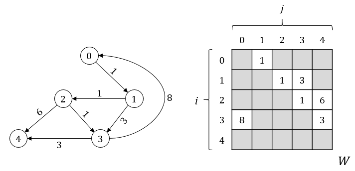
In a weight matrix we can see that cell values are equal to weights between adjacent vertexes. That is why, if we inspect paths from vertex 0 (row 0), we will see that … there is only one path – from 0 to 1. But, on a visual representation we can clearly see paths from vertex 0 to vertexes 2 and 3 (through vertex 1). The reason for this is simple – in an initial state, weight matrix contains distance between adjacent vertexes only. However, this information alone is enough to find the rest.
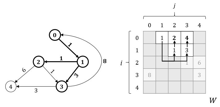
Let’s see how it works. Pay attention to cell W[0, 1]. It’s value indicates, there is a path from vertex 0 to vertex 1 with a weight equal to 1 (in short we can write in as: 0 -> 1: 1). With this knowledge, we now can scan all cells of row 1 (which contains all weights of all paths from vertex 1) and back port this information to row 0, increasing the weight by 1 (value of W[0, 1]).
Using the same steps we can find paths from vertex 0 through other vertexes. During the search, it might happen that there are more than one path leading to the same vertex and what is more important the weights of these paths could be different. An example of such a situation is illustrated on the picture bellow, where search from vertex 0 through vertex 2 revealed one more path to vertex 3 of a smaller weight.
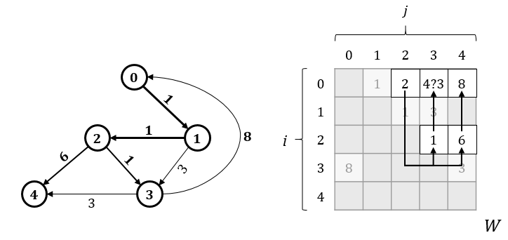
We have two paths: an original path – 0 -> 3: 4 and a new path we have just discovered – 0 -> 2 -> 3: 3 (keep in mind, weight matrix doesn’t contain paths, so we don’t know which vertexes are included in original path). This is a moment when we make a decision to keep a shortest one and write 3 into cell w[0, 3].
Looks like we have just found our first shortest path!
The steps we have just saw are the essence of Floyd-Warshall algorithm. Look at the algorithm’s pseudocode one more time:
algorithm FloydWarshall(W) do
  for k = 0 to N - 1 do
    for i = 0 to N - 1 do
        for j = 0 to N - 1 do
            W[i, j] = min(W[i, j], W[i, k] + W[k, j])
        end for
    end for
  end for
end algorithm
The outermost cycle for on k iterates over all vertexes in a graph and on each iteration, variable k represents a vertex we are searching paths through. Inner cycle for on i also iterates over all vertexes in the graph and on each iteration, i represents a vertex we are searching paths from. And lastly an innermost cycle for on j iterates over all vertexes in the graph and on each iteration, j represents a vertex we are searching path to. In combination it gives us the following: on each iteration k we are searching paths from all vertexes i into all vertexes j through vertex k. Inside a cycle we compare path i -> j (represented by W[i, j]) with a path i -> k -> j (represented by sum of W[I, k] and W[k, j]) and writing the shortest one back into W[i, j].
Now, when we understand the mechanics it is time to implement the algorithm.
Basic implementation
The source code and experimental graphs are available in repository on GitHub.
Author’s note
Before diving into implementation we need to clarify a few technical moments:
- All implementations work with weight matrix represented in form of lineal array.
- All implementations use integer arithmetic. Absence of path between vertexes is represented by a special constant weight:
NO_EDGE = (int.MaxValue / 2) - 1.
Now, let’s figure out why is that.
Regarding #1. When we speak about matrixes we define cells in terms of “rows” and “columns”. Because of this it seems natural to imagine a matrix in form of “square” or “rectangle” (picture 4a).
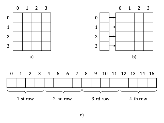
However, this doesn’t necessary mean we have to represent matrix in form of array of arrays (picture 4b) to stick to our imagination. Instead of this, we can represent a matrix in form of lineal array (picture 4c) where index of each cell is calculated using the following formula:
i = row * row_size + col;

// where row      - cell row index,
//       col      - cell column index,
//       row_size - number of cells in a row.
Lineal array of weight matrix is a precondition for effective execution of Floyd-Warshall algorithm. The reason for that isn’t simple and detailed explanation deserves a separate post… or a few posts. However, currently, it is important to mention that such representation significantly improves data locality, which in fact has a great impact on algorithm’s performance.
Here, I am asking you to believe me and just this information in mind as a precondition, however, at the same time I recommend you to spend some time and study the question, and by the way – don’t believe people on the Internet.
Author’s note
Regarding #2. If you take a closer look at the algorithm pseudocode, you won’t find any checks related to existence of a path between two vertexes. Instead, pseudocode simply use min() function. The reason is simple – originally, if there is no path between to vertexes, a cell value is set to infinity and in all languages, except may be JavaScript, all values are less than infinity. In case of integers it might be tempting to use int.MaxValue as a “no path” value. However this will lead to integer overflow in cases when values of both i -> k and k -> j paths will be equal to int.MaxValue. That is why we use a value which is one less than a half of the int.MaxValue.
Hey! But why we can’t just check whether if path exists before doing any calculations. For example by comparing paths both to
Thoughtful reader0(if we take a zero as “no path” value).
It is indeed possible but unfortunately it will lead to a significant performance penalty. In short, CPU keeps statistics of branch evaluation results ex. when some of if statements evaluate to true or false. It uses this statistics to execute code of “statistically predicted branch” upfront before the actual if statement is evaluated (this is called speculative execution) and therefore execute code more efficiently. However, when CPU prediction is inaccurate, it causes a significant performance lose compared to correct prediction and unconditional execution because CPU has to stop and calculate the correct branch.
Because on each iteration k we update a significant portion of weight matrix, CPU branch statistics becomes useless because there is no code pattern, all branches are based exclusively on data. So such check will result in significant amount of branch mispredictions.
Here I am also asking of you to believe me (for now) and then spend some time to study the topic.
Uhh, looks like we are done with the theoretical part – let’s implement the algorithm:
public void FloydWarshall_00(int[] matrix, int sz)
{
  for (var k = 0; k < sz; ++k)
  {
    for (var i = 0; i < sz; ++i)
    {
      for (var j = 0; j < sz; ++j)
      {
        var distance = matrix[i * sz + k] + matrix[k * sz + j];
        if (matrix[i * sz + j] > distance)
        {
          matrix[i * sz + j] = distance;
        }
      }
    }
  }
}
The above code is almost an identical copy of the previously mentioned pseudocode with a single exception – instead of Math.Min() we use if to update a cell only when necessary.
Hey! Wait a minute, wasn’t it you who just wrote a lot of words about why if’s aren’t good here and a few lines later we ourselves introduce an if?
Thoughtful reader
The reason is simple. At the moment of writing JIT emits almost equivalent code for both if and Math.Min implementations. You can check it in details on sharplab.io but here are snippets of main loop bodies:
53: movsxd r14, r14d
// compare matrix[i * sz + j]
//     and distance
56: cmp [rdx+r14*4+0x10], ebx
5b: jle short 64
// if matrix[i * sz + j]
//    greater than distance
//      write distance to matrix
5d: movsxd rbp, ebp
60: mov [rdx+rbp*4+0x10], ebx
64: // end of loop
Assembly code of implementation of innermost loop for of j using if
4f: movsxd rbp, ebp
52: mov r14d, [rdx+rbp*4+0x10]
// compare matrix[i * sz + j]
//     and distance
57: cmp r14d, ebx
// if matrix[i * sz + j]
//    less than distance
//      write value to matrix
5a: jle short 5e
// otherwise
//   write distance to matrix
5c: jmp short 61
5e: mov ebx, r14d
61: mov [rdx+rbp*4+0x10], ebx
65: // end of loop
Assembly code of implementation of innermost loop for of j using Math.Min
You may see, regardless of whether we use if or Math.Min there is still a conditional check. However, in case of if there is no unnecessary write.
Now when we have finished with the implementation, it is time to run the code and see how fast is it?!
You can verify the code correctness yourself by running tests in a repository.
Author’s note
I use Benchmark.NET (version 0.12.1) to benchmark code. All graphs used in benchmarks are directed, acyclic graphs of 300, 600, 1200, 2400 and 4800 vertexes. Number of edges in graphs is around 80% of possible maximum which for directed, acyclic graphs can be calculated as:
var max = v * (v - 1)) / 2;

// where v - is a number of vertexes in a graph.
Let’s rock!
Here are the results of benchmarks run on my PC (Windows 10.0.19042, Intel Core i7-7700 CPU 3.60Ghz (Kaby Lake) / 8 logical processors / 4 cores):
| Method | Size | Mean | Error | StdDev |
|---|---|---|---|---|
| FloydWarshall_00 | 300 | 27.525 ms | 0.1937 ms | 0.1617 ms |
| FloydWarshall_00 | 600 | 217.897 ms | 1.6415 ms | 1.5355 ms |
| FloydWarshall_00 | 1200 | 1,763.335 ms | 7.4561 ms | 6.2262 ms |
| FloydWarshall_00 | 2400 | 14,533.335 ms | 63.3518 ms | 52.9016 ms |
| FloydWarshall_00 | 4800 | 119,768.219 ms | 181.5514 ms | 160.9406 ms |
From the results we can see, calculation time grows dramatically compared to a size of a graph – for a graph of 300 vertexes it took 27 milliseconds, for a graph of 2400 vertex – 14.5 seconds and for a graph of 4800 – 119 seconds which is almost 2 minutes!
Looking at algorithm’s code it might be hard to imagine, there is something we can do to speed up calculations… because well… there are THREE loops, just THREE loops.
However, as it usually happens – possibilities are hidden in details 🙂
Know you data – sparse graphs
Floyd-Warshall algorithm is a base algorithm for solving all-pairs shortest path problem, especially when it comes to dense or complete graphs (because algorithm searches paths between all pairs of vertexes). However, in our experiments we use directed, acyclic graphs, which have a wonderful property – if there is a path from vertex 1 to vertex 2, then there is no path from vertex 2 to vertex 1. For us, it means, there are a lot of non-adjacent vertexes which we can skip if there is no path from i to k.
public void FloydWarshall_01(int[] matrix, int sz)
{
  for (var k = 0; k < sz; ++k)
  {
    for (var i = 0; i < sz; ++i)
    {
      if (matrix[i * sz + k] == NO_EDGE)
      {
        continue;
      }
      for (var j = 0; j < sz; ++j)
      {
        var distance = matrix[i * sz + k] + matrix[k * sz + j];
        if (matrix[i * sz + j] > distance)
        {
          matrix[i * sz + j] = distance;
        }
      }
    }
  }
}
Here are the results of previous (00) and current (01) implementations on the same set of graphs:
| Method | Size | Mean | Error | StdDev | Ratio |
|---|---|---|---|---|---|
| FloydWarshall_00 | 300 | 27.525 ms | 0.1937 ms | 0.1617 ms | 1.00 |
| FloydWarshall_01 | 300 | 12.399 ms | 0.0943 ms | 0.0882 ms | 0.45 |
| FloydWarshall_00 | 600 | 217.897 ms | 1.6415 ms | 1.5355 ms | 1.00 |
| FloydWarshall_01 | 600 | 99.122 ms | 0.8230 ms | 0.7698 ms | 0.45 |
| FloydWarshall_00 | 1200 | 1,763.335 ms | 7.4561 ms | 6.2262 ms | 1.00 |
| FloydWarshall_01 | 1200 | 766.675 ms | 6.1147 ms | 5.7197 ms | 0.43 |
| FloydWarshall_00 | 2400 | 14,533.335 ms | 63.3518 ms | 52.9016 ms | 1.00 |
| FloydWarshall_01 | 2400 | 6,507.878 ms | 28.2317 ms | 26.4079 ms | 0.45 |
| FloydWarshall_00 | 4800 | 119,768.219 ms | 181.5514 ms | 160.9406 ms | 1.00 |
| FloydWarshall_01 | 4800 | 55,590.374 ms | 414.6051 ms | 387.8218 ms | 0.46 |
Quite impressive!
We reduced calculation time in a half! Of course, the denser the graph, the less speed up will be. However, this is one of the optimisations which comes handy if you know in advance what class of data you are intended to work with.
Can we do more? 🙂
Know your hardware – parallelism
My PC is equipped with Inter Core i7-7700 CPU 3.60GHz (Kaby Lake) processor with 8 logical processors (HW) or 4 cores with Hyper-Threading technology. Having more than one core is like having more “spare hands” which we can put to work. So, let’s see which part of work can be efficiently divided between multiple workers and then, parallelise it.
Loops are always the most obvious candidate for parallelisation because in most cases iterations are independent and can be executed simultaneously. In the algorithm, we have three loops which we should analyse and see if there are any dependencies which prevent us from parallelising them.
Let’s start from for of k loop. On each iteration loop calculates paths from every vertex to every vertex through vertex k. New and updated paths are stored in weight matrix. Looking at iterations you might notice – they can be executed in any order: 0, 1, 2, 3 or 3, 1, 2, 0 without affecting the result. However, they still have to be executed in sequence, otherwise some of the iterations won’t be able to use new or updated paths because they won’t be written into weight matrix, yet. Such inconsistency will definitely crush the results. So we need to keep looking.
The next candidate is for of i loop. On each iteration loop reads a path from vertex i to vertex k (cell: W[i, k]), a path from vertex k to vertex j (cell: W[k, j]) and then checks whether known path from i to j (cell: W[i, j]) is shorter than i -> k -> j path (sum of: w[i, k] + w[k, j]). If you look closer at the access pattern, you might notice – on each iteration i loop reads data from k row and updated i row which basically means – iterations are independent and can be executed not only in any order but also in parallel!
This looks promising, so let’s implement it!
Author’s note
for of jloop also can be paralleled. However, parallelisation of innermost cycle in this case is very inefficient. You can verify it yourself by making a few simple changes in the source code.
public void FloydWarshall_02(int[] matrix, int sz)
{
  for (var k = 0; k < sz; ++k)
  {
    Parallel.For(0, sz, i =>
    {
      if (matrix[i * sz + k] == NO_EDGE)
      {
        return;
      }
      for (var j = 0; j < sz; ++j)
      {
        var distance = matrix[i * sz + k] + matrix[k * sz + j];
        if (matrix[i * sz + j] > distance)
        {
          matrix[i * sz + j] = distance;
        }
      }
    });
  }
}
Here are the results of 00, 01 and 02 implementations on the same set of graphs. Parallelisation is done using Parallel class:
| Method | Size | Mean | Error | StdDev | Ratio |
|---|---|---|---|---|---|
| FloydWarshall_00 | 300 | 27.525 ms | 0.1937 ms | 0.1617 ms | 1.00 |
| FloydWarshall_01 | 300 | 12.399 ms | 0.0943 ms | 0.0882 ms | 0.45 |
| FloydWarshall_02 | 300 | 6.252 ms | 0.0211 ms | 0.0187 ms | 0.23 |
| FloydWarshall_00 | 600 | 217.897 ms | 1.6415 ms | 1.5355 ms | 1.00 |
| FloydWarshall_01 | 600 | 99.122 ms | 0.8230 ms | 0.7698 ms | 0.45 |
| FloydWarshall_02 | 600 | 35.825 ms | 0.1003 ms | 0.0837 ms | 0.16 |
| FloydWarshall_00 | 1200 | 1,763.335 ms | 7.4561 ms | 6.2262 ms | 1.00 |
| FloydWarshall_01 | 1200 | 766.675 ms | 6.1147 ms | 5.7197 ms | 0.43 |
| FloydWarshall_02 | 1200 | 248.801 ms | 0.6040 ms | 0.5043 ms | 0.14 |
| FloydWarshall_00 | 2400 | 14,533.335 ms | 63.3518 ms | 52.9016 ms | 1.00 |
| FloydWarshall_01 | 2400 | 6,507.878 ms | 28.2317 ms | 26.4079 ms | 0.45 |
| FloydWarshall_02 | 2400 | 2,076.403 ms | 20.8320 ms | 19.4863 ms | 0.14 |
| FloydWarshall_00 | 4800 | 119,768.219 ms | 181.5514 ms | 160.9406 ms | 1.00 |
| FloydWarshall_01 | 4800 | 55,590.374 ms | 414.6051 ms | 387.8218 ms | 0.46 |
| FloydWarshall_02 | 4800 | 15,614.506 ms | 115.6996 ms | 102.5647 ms | 0.13 |
From the results we can see that parallelisation of for of i loop have reduced the calculation time by 2-4 times comparing to previous implementation (01)! This is very impressive, however, it is important to remember, parallelisation of pure computations consumes all available compute resources which can lead to resource starvation of other applications in the system. Parallelisation should be used with care.
As you might guess – this isn’t the end 🙂
Know your platform – vectorisation
Vectorisation is a transformation of a code operating on a single element into a code operating on multiple elements simultaneously.
This might sound like a complex matter, so let’s see how it works on a simple example:
var a = new [] { 5, 7, 8, 1 };
var b = new [] { 4, 2, 2, 6 };
var c = new [] { 0, 0, 0, 0 };
for (var i = 0; i < 4; ++i)
  c[i] = a[i] + b[i];
In the oversimplified way, execution of iteration 0 of the above for loop on a CPU level can be illustrated as following:
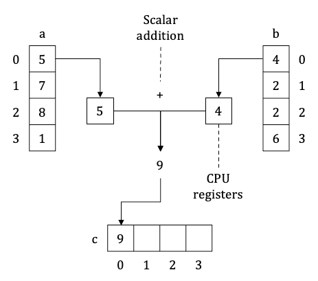
Here is what happening. CPU loads values of arrays a and b from memory into CPU registers (one register can hold exactly one value). Then CPU executes scalar addition operation on these registries and writes the result back into main memory – right into an array c. This process is repeated four times before the loop ends.
Vectorisation means usage of special CPU registers – vector or SIMD (single instruction multiple data) registers, and corresponding CPU instructions to execute operations on multiple array values at once:
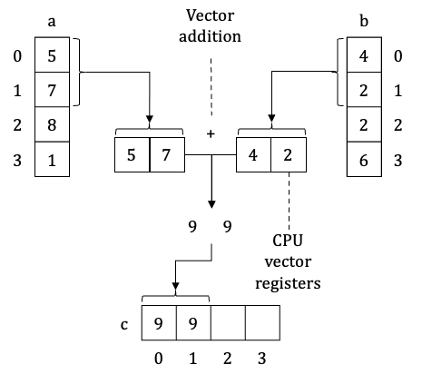
Here is what happening. CPU loads values of arrays a and b from memory into CPU registers (however this time, one vector register can hold two array value). Then CPU executes vector addition operation on these registries and writes the result back into main memory – right into an array c. Because we operate on two values at once, this process is repeated two times instead of four.
To implement vectorisation in .NET we can use – Vector and Vector<T> types (we also can use types from System.Runtime.Intrinsics namespace, however they are bit advance for current implementation, so I won’t use them, but feel free to try them yourself):
public void FloydWarshall_03(int[] matrix, int sz)
{
  for (var k = 0; k < sz; ++k)
  {
    for (var i = 0; i < sz; ++i)
    {
      if (matrix[i * sz + k] == NO_EDGE)
      {
        continue;
      }
      var ik_vec = new Vector<int>(matrix[i * sz + k]);
      var j = 0;
      for (; j < sz - Vector<int>.Count; j += Vector<int>.Count)
      {
        var ij_vec  = new Vector<int>(matrix, i * sz + j);
        var ikj_vec = new Vector<int>(matrix, k * sz + j) + ik_vec;
        var lt_vec = Vector.LessThan(ij_vec, ikj_vec);
        if (lt_vec == new Vector<int>(-1))
        {
          continue;
        }
        var r_vec = Vector.ConditionalSelect(lt_vec, ij_vec, ikj_vec);
        r_vec.CopyTo(matrix, i * sz + j);
      }
      for (; j < sz; ++j)
      {
        var distance = matrix[i * sz + k] + matrix[k * sz + j];
        if (matrix[i * sz + j] > distance)
        {
          matrix[i * sz + j] = distance;
        }
      }
    }
  }
}
Vectorised code can look a bit bizarre, so let’s go through it step by step.
We create a vector of i -> k path: var ik_vec = new Vector<int>(matrix[i * sz + k]). As the result, if vector can hold four values of int type and weight of i -> k path is equal to 5, we will create a vector of four 5’s – [5, 5, 5, 5]. Next, on each iteration, we simultaneously calculate paths from vertex i to vertexes j, j + 1, ..., j + Vector<int>.Count.
Property
Author’s noteVector<int>.Countreturns number of elements ofinttype that fits into vector registers. The size of vector registers depends on CPU model, so this property can return different values on different CPU’s.
The whole calculation process can be divided into three steps:
- Load information from weight matrix into vectors:
ij_vecandikj_vec. - Compare
ij_vecandikj_vecvectors and select smallest values into a new vectorr_vec. - Write
r_vecback to weight matrix.
While #1 and #3 are pretty straightforward, #2 requires explanation. As it was mentioned previously, with vectors we manipulate multiple values at the same time. Therefore, result of some operations can’t be singular i.e., comparison operation Vector.LessThan(ij_vec, ikj_vec) can’t return true or false because it compares multiple values. So instead it returns a new vector which contains comparison results between corresponding values from vectors ij_vec and ikj_vec (-1, if value from ij_vec is less than value from ikj_vec and 0 if otherwise). Returned vector (by itself) isn’t really useful, however, we can use Vector.ConditionalSelect(lt_vec, ij_vec, ikj_vec) vector operation to extract required values from ij_vec and ikj_vec vectors into a new vector – r_vec. This operation returns a new vector where values are equal to smaller of two corresponding values of input vectors i.e., if value of vector lt_vec is equal to -1, then operation selects a value from ij_vec, otherwise it selects a value from ikj_vec.
Besides #2, there is one more part, requires explanation – the second, non-vectorised loop. It is required when size of the weight matrix isn’t a product of Vector<int>.Count value. In that case the main loop can’t process all values (because you can’t load part of the vector) and second, non-vectored, loop will calculate the remaining iterations.
Here are the results of this and all previous implementations:
| Method | sz | Mean | Error | StdDev | Ratio |
|---|---|---|---|---|---|
| FloydWarshall_00 | 300 | 27.525 ms | 0.1937 ms | 0.1617 ms | 1.00 |
| FloydWarshall_01 | 300 | 12.399 ms | 0.0943 ms | 0.0882 ms | 0.45 |
| FloydWarshall_02 | 300 | 6.252 ms | 0.0211 ms | 0.0187 ms | 0.23 |
| FloydWarshall_03 | 300 | 3.056 ms | 0.0301 ms | 0.0281 ms | 0.11 |
| FloydWarshall_00 | 600 | 217.897 ms | 1.6415 ms | 1.5355 ms | 1.00 |
| FloydWarshall_01 | 600 | 99.122 ms | 0.8230 ms | 0.7698 ms | 0.45 |
| FloydWarshall_02 | 600 | 35.825 ms | 0.1003 ms | 0.0837 ms | 0.16 |
| FloydWarshall_03 | 600 | 24.378 ms | 0.4320 ms | 0.4041 ms | 0.11 |
| FloydWarshall_00 | 1200 | 1,763.335 ms | 7.4561 ms | 6.2262 ms | 1.00 |
| FloydWarshall_01 | 1200 | 766.675 ms | 6.1147 ms | 5.7197 ms | 0.43 |
| FloydWarshall_02 | 1200 | 248.801 ms | 0.6040 ms | 0.5043 ms | 0.14 |
| FloydWarshall_03 | 1200 | 185.628 ms | 2.1240 ms | 1.9868 ms | 0.11 |
| FloydWarshall_00 | 2400 | 14,533.335 ms | 63.3518 ms | 52.9016 ms | 1.00 |
| FloydWarshall_01 | 2400 | 6,507.878 ms | 28.2317 ms | 26.4079 ms | 0.45 |
| FloydWarshall_02 | 2400 | 2,076.403 ms | 20.8320 ms | 19.4863 ms | 0.14 |
| FloydWarshall_03 | 2400 | 2,568.676 ms | 31.7359 ms | 29.6858 ms | 0.18 |
| FloydWarshall_00 | 4800 | 119,768.219 ms | 181.5514 ms | 160.9406 ms | 1.00 |
| FloydWarshall_01 | 4800 | 55,590.374 ms | 414.6051 ms | 387.8218 ms | 0.46 |
| FloydWarshall_02 | 4800 | 15,614.506 ms | 115.6996 ms | 102.5647 ms | 0.13 |
| FloydWarshall_03 | 4800 | 18,257.991 ms | 84.5978 ms | 79.1329 ms | 0.15 |
From the result it is obvious, vectorisation has significantly reduced calculation time – from 3 to 4 times compared to non-parallelised version (01). The interesting moment here, is that vectorised version also outperforms parallel version (02) on smaller graphs (less than 2400 vertexes).
And last but not least – let’s combine vectorisation and parallelism!
If you are interested in practical application of vectorisation, I recommend you to read series of posts by Dan Shechter where he vectorised
Author’s noteArray.Sort(these results later found themselves in update for Garbage Collector in .NET 5).
Know your platform and hardware – vectorisation and parallelism!
The last implementation combines efforts of parallelisation and vectorisation and … to be honest it lacks of individuality 🙂 Because… well, we have just replaced a body of Parallel.For from 02 with vectorised loop from 03:
public void FloydWarshall_04(int[] matrix, int sz)
{
  for (var k = 0; k < sz; ++k)
  {
    Parallel.For(0, sz, i =>
    {
      if (matrix[i * sz + k] == NO_EDGE)
      {
        return;
      }
      var ik_vec = new Vector<int>(matrix[i * sz + k]);
      var j = 0;
      for (; j < sz - Vector<int>.Count; j += Vector<int>.Count)
      {
        var ij_vec  = new Vector<int>(matrix, i * sz + j);
        var ikj_vec = new Vector<int>(matrix, k * sz + j) + ik_vec;
        var lt_vec = Vector.LessThan(ij_vec, ikj_vec);
        if (lt_vec == new Vector<int>(-1))
        {
          continue;
        }
        var r_vec = Vector.ConditionalSelect(lt_vec, ij_vec, ikj_vec);
        r_vec.CopyTo(matrix, i * sz + j);
      }
      for (; j < sz; ++j)
      {
        var distance = matrix[i * sz + k] + matrix[k * sz + j];
        if (matrix[i * sz + j] > distance)
        {
          matrix[i * sz + j] = distance;
        }
      }
    });
  }
}
All results of this post are presented bellow. As expected, simultaneous use of parallelism and vectorisation demonstrated the best results, reducing the calculation time up to 25 times (for graphs of 1200 vertexes) comparing to initial implementation.
| Method | sz | Mean | Error | StdDev | Ratio |
|---|---|---|---|---|---|
| FloydWarshall_00 | 300 | 27.525 ms | 0.1937 ms | 0.1617 ms | 1.00 |
| FloydWarshall_01 | 300 | 12.399 ms | 0.0943 ms | 0.0882 ms | 0.45 |
| FloydWarshall_02 | 300 | 6.252 ms | 0.0211 ms | 0.0187 ms | 0.23 |
| FloydWarshall_03 | 300 | 3.056 ms | 0.0301 ms | 0.0281 ms | 0.11 |
| FloydWarshall_04 | 300 | 3.008 ms | 0.0075 ms | 0.0066 ms | 0.11 |
| FloydWarshall_00 | 600 | 217.897 ms | 1.6415 ms | 1.5355 ms | 1.00 |
| FloydWarshall_01 | 600 | 99.122 ms | 0.8230 ms | 0.7698 ms | 0.45 |
| FloydWarshall_02 | 600 | 35.825 ms | 0.1003 ms | 0.0837 ms | 0.16 |
| FloydWarshall_03 | 600 | 24.378 ms | 0.4320 ms | 0.4041 ms | 0.11 |
| FloydWarshall_04 | 600 | 13.425 ms | 0.0319 ms | 0.0283 ms | 0.06 |
| FloydWarshall_00 | 1200 | 1,763.335 ms | 7.4561 ms | 6.2262 ms | 1.00 |
| FloydWarshall_01 | 1200 | 766.675 ms | 6.1147 ms | 5.7197 ms | 0.43 |
| FloydWarshall_02 | 1200 | 248.801 ms | 0.6040 ms | 0.5043 ms | 0.14 |
| FloydWarshall_03 | 1200 | 185.628 ms | 2.1240 ms | 1.9868 ms | 0.11 |
| FloydWarshall_04 | 1200 | 76.770 ms | 0.3021 ms | 0.2522 ms | 0.04 |
| FloydWarshall_00 | 2400 | 14,533.335 ms | 63.3518 ms | 52.9016 ms | 1.00 |
| FloydWarshall_01 | 2400 | 6,507.878 ms | 28.2317 ms | 26.4079 ms | 0.45 |
| FloydWarshall_02 | 2400 | 2,076.403 ms | 20.8320 ms | 19.4863 ms | 0.14 |
| FloydWarshall_03 | 2400 | 2,568.676 ms | 31.7359 ms | 29.6858 ms | 0.18 |
| FloydWarshall_04 | 2400 | 1,281.877 ms | 25.1127 ms | 64.8239 ms | 0.09 |
| FloydWarshall_00 | 4800 | 119,768.219 ms | 181.5514 ms | 160.9406 ms | 1.00 |
| FloydWarshall_01 | 4800 | 55,590.374 ms | 414.6051 ms | 387.8218 ms | 0.46 |
| FloydWarshall_02 | 4800 | 15,614.506 ms | 115.6996 ms | 102.5647 ms | 0.13 |
| FloydWarshall_03 | 4800 | 18,257.991 ms | 84.5978 ms | 79.1329 ms | 0.15 |
| FloydWarshall_04 | 4800 | 12,785.824 ms | 98.6947 ms | 87.4903 ms | 0.11 |
Conclusion
In this post we slightly dived into an all-pairs shortest path problem and implemented a Floyd-Warshall algorithm in C# to solve it. We also updated our implementation to honour data and utilise a low level features of the .NET and hardware.
In this post we played “all in”. However, in real life applications it is important to remember – we aren’t alone. Hardcore parallelisation can significantly degrade system performance and cause more harm than good. Vectorisation on another hand is a bit safer if it is done in platform independent way. Remember some of the vector instructions could be available only on certain CPUs.
I hope you’ve enjoyed the read and had some fun in “squeezing” some bits of performance from an algorithm with just THREE cycles 🙂
References
- Floyd, R. W. Algorithm 97: Shortest Path / R. W. Floyd // Communications of the ACM. – 1962. – Vol. 5, №. 6. – P. 345-.
- Ingerman, P. Z. Algorithm 141: Path matrix / P. Z. Ingerman // Communications of the ACM. – 1962. – Vol. 5, №. 11. – P. 556.
History
- 2022/05/11 – Updated post category to “Book of All-pairs Shortest Paths”.

2 thoughts on “Implementing Floyd-Warshall algorithm for solving all-pairs shortest paths problem in C#”